1.43× Faster MoE Training: LoongForge Redefines EP Expert Load Balancing with Topology-Aware Optimal Transport

MoE is now the default architecture for frontier models, and the direction of the next generation is clear: more experts, sparser activation. DeepSeek-V4-Pro raised the number of routed experts per layer from 256 in V3 to 384, while the number of experts activated per token actually dropped from 8 to 6.

Those architectural gains come at a price: the complexity moves into the training system. How many tokens each GPU has to process depends entirely on routing results, and the more numerous and fine-grained the experts, the harder the routing tail is to predict. As soon as a few experts become hotspots, tokens pile up on the ranks hosting them, stretching out the step time while every other rank sits idle waiting even after finishing early.

So in our experience, when MoE training is slow, the root cause is usually not "the GPUs aren't fast enough" or "the network isn't wide enough" — it's whether load can be rebalanced in time.

The field arrived at an obvious remedy early on: temporarily replicate a hot expert's weights onto some idle rank and let that idle GPU take over part of the token computation. FasterMoE, Echo in Megatron, DeepSeek's LPLB, and the recent ICML 2026 work LLEP are all representatives of this idea.

Within a single node this is natural: GPUs talk over NVLink, so it hardly matters which idle GPU you move the weights to. But the scale of the new generation of models already forces the EP domain across nodes: hundreds of experts' weights have to be spread out by expert parallelism, and NVIDIA's reference training configuration for V4-Pro calls for EP64 across 64 nodes — 512 H100s in total. Once the EP domain leaves a single node, "which idle GPU" is no longer an equivalent choice: intra-node is NVLink, cross-node goes over InfiniBand, and the cost of shipping one hot expert's weights can differ by an order of magnitude.

The problem we see is that most of these approaches optimize for exactly one thing — flatten the load as much as possible — and implicitly treat idle capacity as a homogeneous resource, as if one idle GPU were interchangeable with another. The result is that whether expert weights end up moved to a different node becomes the dominant factor in communication cost: two plans with nearly identical load-balance quality can have wildly different real overhead.

In other words, replica placement cannot only ask "where is there room?" — it also has to ask "how expensive is it to move there?"

Based on that observation, we wrote this work up as a paper, now on arXiv: TAOT: Topology-Aware Optimal Transport for Dynamic Expert Replica Placement in MoE Training (arXiv:2608.03676). The method we propose, TAOT (Topology-Aware Optimal Transport), is the first to bring both the peak-shaving benefit and the cost of moving weights across nodes into a single optimization objective, using optimal transport to decide which GPU each hot expert's replica should land on. The trade-off — prefer intra-node, go cross-node when necessary — is expressed directly inside the optimization, which fits multi-node EP settings with micro-batch-level dynamic hotspots.

• Technical report: https://arxiv.org/abs/2608.03676
• Project: https://github.com/baidu-baige/LoongForge

1. Why We Think Load Balancing Alone Isn't Enough

Consider a typical replica mechanism: reserve a few empty slots on lightly loaded ranks (we call them guest slots in the paper), copy a hot expert's weights into one of them, and let that light rank take over part of the token computation. The routing target doesn't change; the computation simply happens somewhere else.

What matters is which GPU you copy to. Existing strategies typically optimize only for "best load balance," treating every free slot as an identical resource. But intra-node NVLink and cross-node IB/RDMA are not in the same league in effective bandwidth or cost. So two plans with nearly identical peak-shaving quality can differ substantially in end-to-end communication cost, purely because one kept the weights inside the node and the other shipped them next door.

The closest work to TAOT is DeepSeek's LPLB. It models the assignment of tokens to free slots as a linear program, but constrains replica communication paths using predefined graph structures such as Cube, Hypercube, and Torus. That works well at small scale when hotspots happen to fall on adjacent edges of the graph. But once EP scale grows, or hotspots don't line up with the fixed topology, nearby capacity is exhausted quickly while distant idle ranks are shut out of the feasible region by the graph — and the overall scheduling space shrinks noticeably.

Our approach inverts this: instead of relying on a fixed topology graph, we use a continuous communication cost matrix plus a soft topology preference. Placing nearby is preferred, but when there truly isn't room inside the node, cross-node remains a "legal but more expensive option" rather than being cut off outright. This is much closer to the micro-batch-level fluctuating hotspot distribution we observe in real multi-node EP.

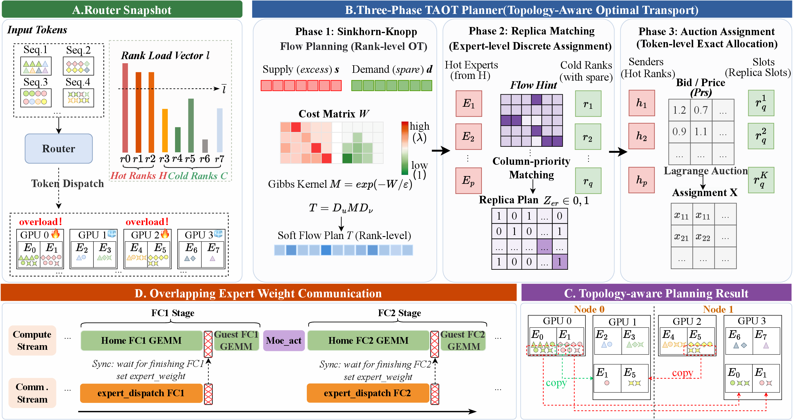
2. Three-Phase Planning: From "Where Should It Flow" to "Who Sends How Much"

Solving for balance and communication cost jointly in one shot makes the problem size blow up with EP degree. So we decompose it into the three interlocking, progressively refined phases shown below.

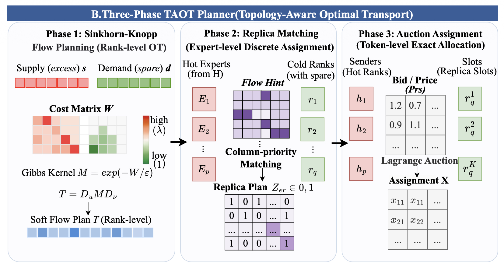
Phase 1: Sinkhorn-Knopp topology-aware flow planning (rank level). We treat each rank's overload as "supply" and its free capacity as "demand," then solve an optimal transport problem under the topology cost matrix W. In essence it answers: globally, which hot ranks' overload should be moved to which cold ranks to be worthwhile. Vanilla OT requires a linear program, which is awkward on GPU; after relaxing with a negative-entropy regularizer, the optimum takes a Gibbs kernel form:

T = diag(u) · M · diag(v)

which can be computed with just a few alternating rounds of Sinkhorn-Knopp GEMV iterations — far friendlier to a GPU implementation. When we set the regularization coefficient to the cross-node cost λ, the ratio of intra-node to cross-node kernel values is exactly greater than 1. That is where the "soft topology preference" comes from mathematically: cross-node is not forbidden, it just has to carry a higher cost.

Phase 2: Column-first iterative matching (expert level). Phase 1 gives a continuous flow reference, but replica placement is ultimately an integer decision: each cold rank holds at most K complete replicas, and several cold ranks may pick the same hot expert. In this phase we score every (cold rank, hot expert) pair with a three-tier score — the primary term is how many tokens this match can offload (balance benefit), the second is topology preference, and only the third is Phase 1's OT flow hint (used as a global reference only to break ties). The key trade-off here: if the outer loop iterates over experts (row-first), heavily loaded experts tend to fill up slots first, light ranks don't get enough scheduling opportunity, and we measured residual imbalance as high as 7–10%. Switching to column-first matching from the cold rank's perspective — each round, every cold rank independently picks its best-fitting expert, conflicts are arbitrated, and ranks that miss out go to the next round — pushed residual imbalance down to 1–2%.

Phase 3: Lagrangian auction token assignment (token level). Phase 2 fixes "how many tokens expert e plans to give slot s," but e's tokens are actually scattered across several ranks, so we still need to compute how many each source rank sends. Splitting proportionally introduces floating-point truncation error and ignores topology information. We introduce a Lagrange multiplier (a price) on each rank's capacity constraint: each round, every slot bids on net benefit — topology benefit minus current price — and the winning rank's price rises, naturally decaying its competitiveness in the next round. This folds topology preference into the assignment, spreads load more evenly, and — because the iteration count is fixed — is inherently compatible with CUDA Graph.

3. Online Planning Must Not Become the New Bottleneck: Fusing Hundreds of Kernels into a Few

Three-phase planning is not lightweight — it involves optimal transport, column-first matching, and auction bidding. But TAOT has to run in real time, every micro-batch: if planning itself is too expensive, the savings on the communication side are easily cancelled out. Keeping planning under 1% of a single forward-backward (F+B) pass takes more than algorithm design; it takes a layer of easily overlooked kernel-level engineering.

The problem shows up mainly at small scale. At EP8 or EP16, the planner's actual GPU work is tiny, yet a naive PyTorch implementation triggers a swarm of small kernels on every call: rebuilding tensors, running 50 Sinkhorn rounds, looping K rounds of Phase 2 — hundreds of launches in total. Host-side launch overhead ends up far exceeding the GPU's real compute time, and the planner itself risks becoming the new bottleneck.

We rewrote the whole thing in Triton, cutting those hundreds of launches down along three directions:

• Static tensor caching. The topology cost matrix M, each expert's home rank, and topology preferences depend only on the topology configuration (R, E, GPUs per node, cross-node cost) — not on how tokens are distributed — and stay constant throughout training. The original implementation rebuilt them every time, adding roughly 15 extra kernel launches. We cache them in a process-level dictionary; after the first call it's a straight hit, and those 15 launches disappear.
• Single-CTA Sinkhorn kernel for Phase 1. 50 rounds of Sinkhorn-Knopp were originally 50 torch.mv + clamp calls, about 150 launches. Since R ≤ 64, all of M, u, and v fit in registers, so we packed all 50 iterations into a single CTA, fully unrolled at compile time — 150 launches become 1, with no CPU-GPU synchronization in between.
• Fusing Phase 2's K rounds. We fuse K rounds of assignment into one launch, keeping the used[E,R] mask entirely in registers across rounds without writing back to global memory until the very end. There's a counter-intuitive trade-off here: we deliberately do not unroll the inner R iterations at compile time — unrolling replicates the [E,R] temporary tensor R times, blowing out registers and collapsing SM occupancy at EP16. Using a dynamic loop instead lets the compiler reuse registers across rounds, and occupancy recovers markedly.

The algorithm determines planning quality; kernel optimization determines whether it can run in real time in a per-micro-batch setting. Together, they let TAOT achieve better balance while keeping online planning overhead under 1% of forward time.

4. Planning Isn't Enough — the Communication Has to Be Hidden Too

Having brought cross-node communication down, we went one step further: the remaining cost of distributing optimized guest expert weights is hidden inside the home expert computation on the same GPU, as shown below.

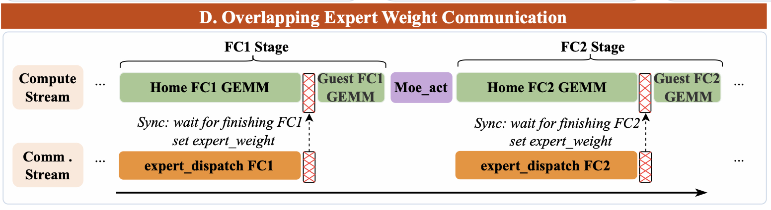
The backward pass works the same way: weight gradients computed by guest experts are sent back to the home rank for accumulation through one reverse All-to-All. The extra communication introduced by the guest expert mechanism is thus largely masked by computation.

5. Measured Results: Faster Training, Cheaper Communication

① End-to-end: 1.43× speedup with no accuracy impact

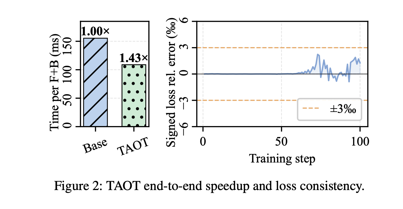
The speedup comes from better load balance plus effectively hidden expert communication — not from trading away numerical accuracy. The guest expert path neither changes the target-expert semantics of any token, nor drops gradients: in the backward pass guest gradients are faithfully sent back and accumulated onto the home expert.

② Balance quality and communication cost, viewed separately

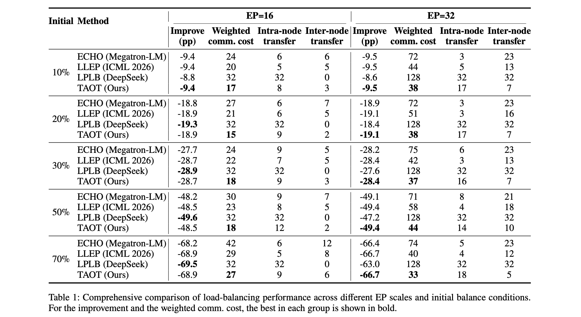
We deliberately did not collapse the two metrics into a single score. End-to-end, expert communication and computation stand at roughly a 1:7 ratio, so even if two plans differ by just 1pp in imbalance, about a 7% drop in communication offsets the cost of the compute tail. And the larger EP gets, the shorter each GPU's compute window and the higher the communication share — pushing that break-even point down further. Presenting balance quality and communication cost separately makes the real trade-offs easier to judge.

• Balance quality: at EP=16 TAOT is a solid second, trailing LPLB by about 1pp — but that 1pp buys a communication reduction that matters more end-to-end. At EP=32 it takes the lead, best or tied-best in every scenario. LPLB degrades noticeably from EP=16 to EP=32: Torus 4×8 restricts migration paths to adjacent edges, so as scale grows and hotspots scatter, nearby capacity runs out first while distant idle GPUs can't participate in scheduling. Our soft preference behaves in exactly the opposite way — the larger EP is, the more low-load ranks there are, and the larger the offload candidate space becomes.
• Communication cost: TAOT is the lowest across all ten configurations. At EP=16 it lands at 15–27, up to 53% below LPLB's fixed 32; at EP=32 it lands at 33–44, up to 55% below ECHO and up to 74% below LPLB. The comparison against LLEP makes another point: the same target imbalance does not imply the same communication efficiency. At 70% imbalance with EP=32, TAOT's cost is 33 versus LLEP's 40 — the difference being that we write intra-node/cross-node cost directly into the placement decision, preferring capacity that is cheaper to communicate with.

③ Scalability and overhead: the larger the scale and the higher the initial imbalance, the bigger the gain

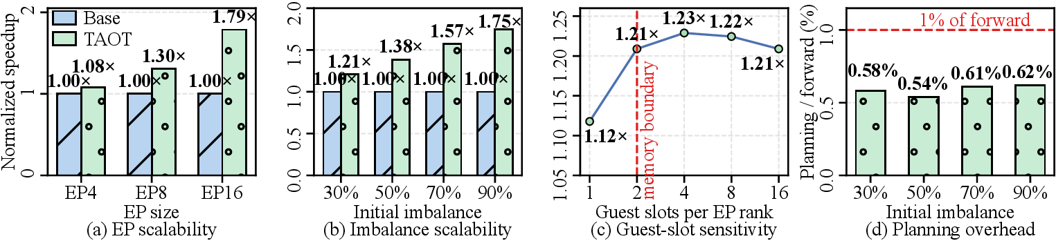
Three trends are clear: the larger the EP scale, the larger the speedup (a bigger parallel domain offers richer global idle capacity); the more imbalanced the start, the larger the speedup (a longer hotspot tail means more load the guest mechanism can offload); and online overhead stays under 1% of forward time, without growing linearly with imbalance — low enough to use every micro-batch, and unlikely to turn into a new bottleneck.

④ Ablation: both components do distinct work, and neither is dispensable

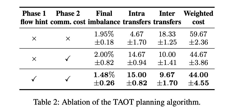
At EP=32 with 70% initial imbalance, we treat Phase 1's flow hint and Phase 2's communication cost modeling as two switches:

• With only Phase 2, cross-node transfers drop from 18.33 to 10.00 and weighted cost from 59.67 to 44.67, while imbalance holds steady at about 2% — showing that it prefers placing replicas inside the node while preserving peak-shaving capability.
• Adding Phase 1 on top, imbalance falls further from 2.00% to 1.48%, and communication cost drops along with it — the rank-level flow hint acts as a global reference, avoiding the unreasonable paths that column-first matching's local greediness would otherwise produce.

Together they form a better balance-versus-communication trade-off.

6. What We Set Out to Fill In: An Underrated Link in MoE Balancing

Placing TAOT back on the map of MoE load balancing makes its position fairly clear.

Over the years, MoE balancing research has covered strategy switching (SmartMoE), capacity prediction (EfficientMoE, DynamicMoE), expert replication (FasterMoE, Echo, LLEP), expert relayout, and more — but few approaches write both the peak-shaving benefit and the cost of moving weights into the objective function. Some depend on a fixed, complex communication paradigm (LAER-MoE); some confine balancing to a single node (FEPLB, which relies on Hopper's NVLink Copy Engine); some constrain paths with a hard topology graph (LPLB).

We target the more general standard EP setting: no special hardware, no lock-in to a single node, no predefined graph. Instead, a continuous cost matrix and a soft topology preference express the trade-off — prefer intra-node placement, go cross-node when necessary — directly in the optimization objective. What it fills in is precisely the piece that has stayed underrated while mattering a great deal to end-to-end cost: where a replica goes was never only a question of where there's room.

For MoE training, where expert counts and EP scale keep growing, we believe this kind of topology-aware real-time replica planning is likely to move from a point optimization to a more fundamental system capability. Which turns the question into: can it land stably inside a training framework, so users can simply enable it in real training jobs?

7. From Paper Method to a Usable Framework Capability

On paper, TAOT is a planning method for "where should an expert replica go." Inside a real training system it also needs topology information, online solving, weight distribution, compute-communication overlap, and a training entry point to work together. That is exactly why we did not ship TAOT as a standalone algorithm, but folded it into our open-source omni-modal training framework LoongForge as an extension of the MoE expert mechanism.

🔗 LoongForge on GitHub: https://github.com/baidu-baige/LoongForge

LoongForge evolved from Baidu Baige's AIAK-Training-LLM acceleration suite. Before open-sourcing, it had already provided production-grade training support to enterprise customers across large language models, computer vision, and embodied intelligence — typically 30%–50% faster than the customer's baseline, with the largest production job exceeding 5,000 XPUs. We target the more general training-engineering problem: one framework covering LLM, VLM, VLA, and Diffusion scenarios, spanning the mainstream pretraining-to-SFT pipeline, validated over a long period across GPU and Kunlun XPU platforms, thousand-GPU clusters, and many kinds of real production workloads.

Making all these model classes fast with a single engine isn't realistic. Our approach splits the backend into two stacks by modality: LLM / VLM / Diffusion run on a deeply customized Megatron-LM, taking full advantage of its mature TP/PP/EP/CP parallelism; embodied models such as VLA and world-action models (WAM) are decoupled from Megatron and run on a torch-native DDP / ZeRO-1 / FSDP / HSDP stack — these models aren't large in parameter count, but their action heads and multi-view inputs are structurally complex, and the native stack is simply more flexible for them. Both stacks are deeply optimized, each aiming to beat the mainstream open-source baseline in its own domain. TAOT is one of the optimizations that lands in the former: you don't need to reproduce the paper's three-phase planner yourself — when you hit expert load skew and cross-node communication bottlenecks, just turn it on in the config.

Beyond "running fast," a framework also has to make "onboarding fast." LoongForge ships standard components for 20+ model families and nearly 40 concrete models: LLMs including DeepSeek-V3/V4, Qwen3/Qwen3-Next, GLM-5, MiniMax, and MIMO; VLMs including Qwen3-VL, InternVL3.5, LLaVA-OneVision-1.5, ERNIE4.5-VL, and Kimi-K2.5; diffusion models including Wan2.1/2.2 and Qwen-Image; and embodied models including Pi0.5, GR00T-N1.6/N1.7, xVLA, FastWAM, and LingBot-VA. The model layer is decomposed into abstractions such as Encoder, Foundation, and composition scheduling, so ViT and LLM components can be swapped freely, and much of the adaptation work can be done through YAML for module composition and strategy configuration — onboarding a new model doesn't mean rebuilding a training stack from scratch.

If you're running large-scale MoE training and a handful of hot experts are dragging out your step time, give LoongForge a try — and feel free to reach us through GitHub Issues.

• Paper: https://arxiv.org/abs/2608.03676
• GitHub: https://github.com/baidu-baige/LoongForge